In Part 1 of this post, we used the idea of shining a light through a cut-out in a piece of paper and discussed how the projection of light onto a dark surface can be used to get an idea of the paper’s inclination. In Part 2, we will begin introducing some of the mathematics involved in using values provided by an accelerometer (like looking at the shape of the light projection) to calculate the inclination of the accelerometer. For now, we’ll just focus on a single-axis example so that we can illustrate the derivation process; then, in Part 3, we’ll extend the mathematics to a three-axis application in the context of an MWD application.
The Math
The math behind calculating inclination can get a little bit confusing, so we’ll take it one baby-step at a time. At the core of inclination calculations is the idea of a ‘vector projection’ (remember our analogy with the light projection onto the surface?), so we’ll begin with a quick review of what that is. In the discussion that follows, prior knowledge of things like what a vector is and how to trigonometry is assumed; if this is your first time seeing those words, you may want to spend some time brushing up on those concepts.
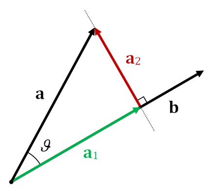
The concept of a vector projection is most easily explained with a picture. The picture below is something I found on the aptly titled Wikipedia page, ‘Vector projection.’ The picture shows two vectors, a and b, and it shows the vector projection of vector a onto vector b. The projection itself is shown by the green vector, denoted as vector a1. Think of it this way: Vector b is like a surface and vector a is like a slot on a piece of paper and, if a light was shining through a, the length of the light that would be projected onto b is shown by a1 (since the light is being projected onto b, the direction of a1 is, by definition, the same as b). Now let’s see how we can use this information in an accelerometer application.
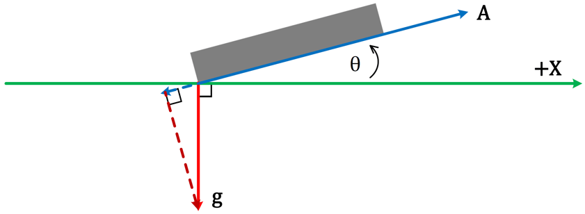
Take a look at the picture below (I drew it myself. I used different colors than the Wikipedia picture, don’t let that confuse you.) The red vector, g, is the gravity vector (it’s magnitude and direction are known); the blue vector, A, is the sensitive axis of the accelerometer. The green line represents the surface of the earth (I chose green because grass is green) and it also represents our frame of reference (that’s what the +X is). Ultimately, it’s the angle between the green line and vector A (denoted by θ) that we want to calculate. That’s the inclination. (Right now, we’re just considering a single axis – baby-steps and all that).
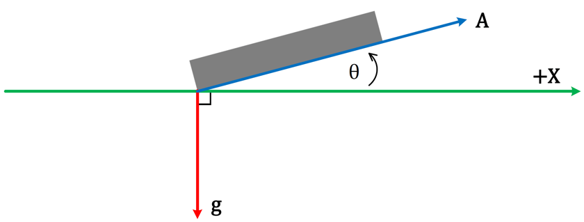
At this point, you may have guessed that calculating inclination is going to involve a vector projection. As it turns out, the acceleration value reported by the accelerometer is the magnitude of the projection of vector g onto vector A (this value can also be called the ‘scalar projection of g onto A’).
The challenge here is to find an equation that uses the information we know (we know all about gravity and the accelerometer tells us the scalar projection of gravity onto its sensitive axis) to calculate our inclination. However, before doing that, let’s address some of the differences between my picture of the accelerometer and Wikipedia’s example picture.
My picture looks a little bit different than Wikipedia’s example picture: The angle between my two vectors, α, is greater than 90°, which makes visualizing the projection a little less obvious. Fortunately, this is easy enough to address by redrawing my picture.
The blue dotted line shows the vector projection of g onto A. In the case where the angle between two vectors is greater than 90° (but less than 180°), the projection vector is going to have an opposite direction with respect to the vector onto which it is projected. Just to make things a little clearer, I redrew our picture and included only the important stuff.
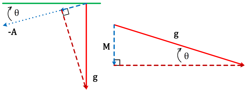
The left half of our redrawn picture shows a close-up of the gravity-projection triangle and the right half of the picture shows the triangle re-positioned with some labels added. The vector projection of g onto A is denoted as vector M. The angle shown in the triangle, θ, is the same angle between the accelerometer and the surface of the earth shown in my first picture (you can use basic properties of intersecting lines and triangles to see that the two angles are the same).
Let’s not forget that our objective is to find the value of θ based on the information we know. Looking at our triangle, if we know the magnitude of g and the magnitude of M, we can use some basic trigonometry to find our angle of inclination. The magnitude of g is easy – that’s just the magnitude of the gravity vector and we know that that’s the same everywhere: g=9.81 m/s2 or g=1 g. The magnitude of M, denoted by M (the vector is with bold typeface, but its magnitude is not), is easy too – that’s just the measurement that the accelerometer gives us. Now, let’s use a little trigonometry to tie it all together:
.png?width=658&name=Screenshot%20(65).png)
The purpose of this blog post was to give a very basic example of how to use the readings from an accelerometer as well as information about gravity to derive an equation that tells us something about inclination. To that effect, I decided to keep things as simple as possible at the expense of mathematical rigor (for example, I never really mentioned that, if the accelerometer readings and the magnitude of gravity are in units of g-force, then the angle of inclination in the above equation is given in radians – details, whatever). Additionally, we didn’t really get into any of the nuances of calculating inclination (such as accelerometer resolution, incremental sensitivity, instabilities of the inverse sine function, etc). All that to say that there is a lot of information that is beyond the scope of these blog posts, but I hope the information presented so far has been a helpful starting point.